Abstract
Can I represent text with a small number of understandable features and still retrieve relevant documents? In this study, I used JEV to assess 34 fixed features for each of the 13,083 messages in BANKING77. The 10,003 training messages became the retrieval corpus, and the 3,080 test messages served as queries. A result was considered relevant when it had the same intent label as the query.
Cosine similarity between the feature vectors retrieved a correct first result for 83.67% of queries, compared with 80.10% for BM25. The difference was 3.57 percentage points, with a paired 95% bootstrap interval of 1.92–5.26 percentage points. Ordinary and weighted dot product performed substantially worse: 25.97% and 28.02%, respectively.
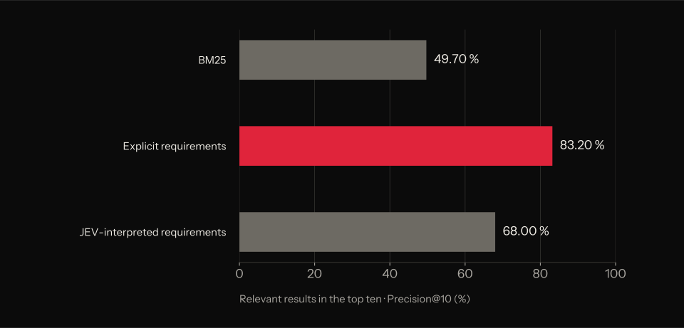
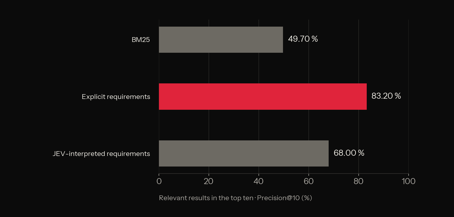
In a separate evaluation of 100 query formulations across 25 semantic groups, explicitly specified feature requirements achieved a Precision@10 of 83.20%. When JEV interpreted the query into requirements, the result was 68.00%, compared with 49.70% for BM25. This evaluation uses relevance derived from dataset labels, rather than independent human judgments of each result.
The results show that a small, named feature space can preserve useful retrieval information in this domain. They also show that the representation and ranking method must be evaluated together. The study does not compare against a conventional embedding model and therefore does not establish that jevbeddings can generally replace such models.
What if the numbers had names?
Imagine searching for messages about cards that have not arrived. A search system returns a list. The first result looks relevant, but why is that particular document at the top?
Texts can be compared by representing them as sequences of numbers. I wanted to test how well retrieval would work if I decided in advance what each number should mean.
One dimension might describe whether the message concerns a payment card. Another might indicate that the card has not arrived. A third might represent the customer asking for a status update. I could then examine which features moved a document up the ranking and which moved it down.
That was the idea behind testing Jevbeddings. I had JEV assess the texts using a fixed set of questions and used the answers as vectors for retrieval. I then tried several ways of comparing those vectors to see how well they worked.
What I liked about this setup was being able to inspect which features influenced a result. The model's assessment was still something I had to trust or check against the text, but I could calculate the contributions to the ranking.
I wanted to investigate three things in particular: How much information do 34 such features preserve? How should the vectors be compared? And what happens when I use the features as explicit search requirements, with the ability to deprioritize or filter out particular results?
From a message to 34 numbers
I defined four feature groups:
| Group | Count | Examples |
|---|---|---|
| What the message concerns | 10 | Cards, cash, transfers, identity verification |
| Event or problem | 12 | Failed payment, extra fee, card not received |
| What the customer wants | 6 | Cancel, get a refund, change something, get a status update |
| State | 6 | Pending, declined, missing, incorrect, unrecognized, expired |
For each text, I asked jev-1.13.0 the same 34 questions. Each answer is a value between 0 and 1. Together, the answers form a vector of 34 numbers.
Think of each number as the model's assessment of how well the text satisfies the corresponding feature. I do not have human ground-truth values for every feature. I therefore do not interpret, for example, 0.9 as an established 90% probability that the feature is correct.
Here are six values for an actual test message:
I still have not received my new card, I ordered over a week ago.
| Feature | Value |
|---|---|
| Concerns a card | 0.99 |
| Card not received | 0.98 |
| Something is missing | 0.98 |
| Wants a status update | 0.97 |
| Waiting for something to complete | 0.97 |
| Something is incorrect | 0.78 |
I can read the representation and consider whether it seems reasonable. The last value is also a reminder that a clear label does not automatically produce an unambiguous assessment. Does a delay mean that something is “incorrect”? The definition and the model's interpretation determine the numbers I get.
All definitions and exact questions are in the feature schema.
How I set up the test
I used BANKING77, introduced by Casanueva and colleagues in 2020. The dataset consists of English banking queries across 77 categories.
I followed the official split: 10,003 messages as documents and 3,080 as queries. Each query was compared with every document. The categories were used to evaluate retrieval, not to train a classifier.
JEV received only the message text and the fixed feature questions, without category names or labeled examples. The 34 features were not paraphrases of the 77 categories, but the schema was designed for banking messages and therefore had some topical overlap.
The schema and protocol were frozen and checksummed before the test file was downloaded. The supplemental queries were created from the training set's category inventory and frozen before test results were examined. No parameters were fitted to test results. The timestamps were local, not a public preregistration.
In the main test, queries and documents were assessed in the same way. A high value means that a feature is present in the message, not necessarily that the user wants to prioritize it. Later, I also tested explicit search requirements, which use the numbers differently.
Four ways to rank
I compared three ways of ranking the JEV vectors, alongside BM25 on the original text. In the formulas below, contains the query values and the document values.
Dot product: sum the overlap
The simplest calculation multiplies the values for each feature and sums their contributions:
If both the query and the document score highly on “card not received,” the contribution is large. If either scores low, the contribution is small. Each feature has its own contribution that I can display.
A document with high values across many features can gain an advantage even if it does not match the query particularly precisely.
Cosine: compare the direction
Cosine similarity divides the dot product by the lengths of both vectors:
The pattern of features then matters more than their overall magnitude. Length here means the vector's magnitude, not the number of words in the text.
A constructed example: the query is [1; 0.5; 0], document A is [0.9; 0.45; 0], and B is [1; 1; 1]. Dot product gives A 1.125 and B 1.5. With cosine, A gets 1 and B approximately 0.775. A wins because its features have the same proportions as the query.
Cosine therefore does not distinguish between weak and strong values that have the same proportions. Whether that is desirable depends on the task.
Same vectors. Different winner.
The query is q = [1; 0.5; 0]. Switch the calculation to see what happens to the two documents.
[0.9; 0.45; 0]
[1; 1; 1]
B wins with dot product.
Weighted relevance: give rare features more weight
Some features occur in many documents. I therefore also tested a dot-product variant that gives rare features more weight. The weights were calculated using only the training documents, with 0.5 as the threshold for a feature being present.
The score was normalized by a value that is identical for every document in a given query. This does not change the ordering: the difference from ordinary dot product comes from the feature weights. The exact calculation is in the ranking code.
BM25: a word-based reference
BM25 searches the text directly, gives rare words more weight, and adjusts for document length. I used k1 = 1.2 and b = 0.75. Text was lowercased and split into words and numbers, without stemming or stop-word removal.
This gives me a concrete reference: what do the model assessments add compared with searching the words directly?
What counts as a good result?
The primary metric was Top-1: the fraction of queries for which the first document had the same category as the test message. I also measured whether at least one of the first five results was relevant, called Hit@5.
Hit@5 is not the same as Recall@5. If the corpus contains 100 relevant documents and I find four of them among the first five, Precision@5 is 80%, Recall@5 is 4%, and Hit@5 is 1 for that query.
I also measured MRR, which rewards the first relevant result appearing early in the ranking, and nDCG@10, which evaluates the positions of relevant results among the first ten. In every case, relevance was determined by the dataset category.
The result: ranking made a large difference

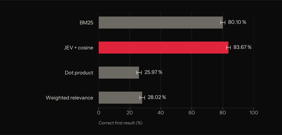
| Method | Top-1 | Hit@5 | Precision@5 | Recall@5 | MRR | nDCG@10 |
|---|---|---|---|---|---|---|
| BM25 | 80.10% | 93.80% | 70.34% | 2.93% | 0.8611 | 0.6769 |
| JEV + cosine | 83.67% | 93.60% | 78.44% | 3.22% | 0.8802 | 0.7678 |
| JEV + dot product | 25.97% | 49.61% | 29.99% | 1.08% | 0.3715 | 0.3025 |
| JEV + weighted relevance | 28.02% | 49.81% | 31.86% | 1.16% | 0.3863 | 0.3203 |
All three vector methods used exactly the same saved JEV assessments. Their differences come from the calculation that ranks the documents.
Cosine achieved a Top-1 score 3.57 percentage points higher than BM25. I estimated the difference using 2,000 paired bootstrap resamples: in each resample, both methods used the same sampled test messages. The interval was 1.92–5.26 percentage points. I made no correction for multiple comparisons. The interval describes variation across the messages in this benchmark, not certainty that the same improvement will occur in another domain.
BM25 had a marginally higher Hit@5. Cosine therefore did not win on every metric, but it placed a relevant document first more often and had higher precision among the first five.
I also checked for overlap between training and test texts. After normalizing case and whitespace, I found seven test messages that also appeared in the training set. Without them, Top-1 was 83.63% for cosine and 80.05% for BM25. The overall picture was therefore unchanged.
Why did dot product perform so poorly?

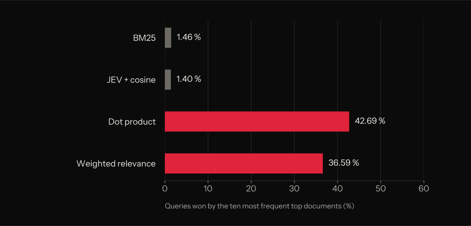
After the main test, I examined which documents repeatedly ranked first. I did not change the method based on this analysis.
| Method | Distinct first-place documents | Share of queries won by the ten most frequent winners | Average strong features in the winning document |
|---|---|---|---|
| BM25 | 2,383 | 1.46% | 4.69 |
| Cosine | 2,456 | 1.40% | 4.75 |
| Dot product | 232 | 42.69% | 10.39 |
| Weighted relevance | 255 | 36.59% | 10.05 |
A “strong feature” here means a value of at least 0.5. The average document had 4.96 such features.
With dot product, just ten documents won almost 43% of all queries. The winners also had far more strong features than the average document. This fits the weakness suggested by the formula: high values across many features can give a document a large advantage.
This is a descriptive association, not isolated proof of the cause of each error. It does, however, provide a concrete explanation to investigate further. Weighted relevance reduced the problem somewhat but remained far behind cosine on this task.
I can also inspect what happened in one incorrect result. The query “How do I locate my card?” had the ground-truth category card_arrival. Weighted relevance retrieved a message about a card lost at a restaurant, with concerns about unauthorized use.
The largest raw contributions came from “card not received” at 2.94, “security concern” at 1.04, and “concerns a card” at 0.85. I can therefore see which assessments produced the result. The query itself is also ambiguous without more context. The label gives me a consistent evaluation rule, but it is not necessarily the only reasonable interpretation of every message.
When the query describes what I want to find

The main test compared one customer message with other customer messages. But a query can also be a request: find transfer problems. Find fees. Find cards that have not arrived.
Here, I can specify which features should matter instead of treating the query as another customer message. I created 25 semantic groups with four formulations each, for a total of 100 queries. For each group, I defined both relevant categories and explicit feature weights.
For card-delivery queries, for example, the requirements were weight 1 on “concerns a card,” weight 1 on “card not received,” and weight 0.5 on “wants a status update.” The same explicit requirements were used for all four formulations in the group.
I compared BM25, the manually specified requirements, and a variant in which JEV interpreted the natural-language query into requirements.
| Method | Precision@10 | Hit@10 | MRR | nDCG@10 |
|---|---|---|---|---|
| BM25 | 49.70% | 92.00% | 0.6823 | 0.5110 |
| Explicit feature requirements | 83.20% | 92.00% | 0.8854 | 0.8372 |
| JEV-interpreted query requirements | 68.00% | 83.00% | 0.7000 | 0.6721 |
The difference between the last two rows shows why interpretation and ranking should be evaluated separately. With explicit requirements, I know which weights the query should use. With natural language, the model must also identify them. Six of the 100 interpreted queries were held for review because of unsupported concepts, uncertain requirements, or a lack of active requirements. They count as zero retrieval in the results.
This is a limited test. Relevance was determined through groups of existing categories, and the feature requirements were created as part of the same task setup. I do not have independent human judgments for all queries and documents. The four formulations in each group are also closely related. The result represents 25 constructed retrieval tasks, not 100 independent information needs.
Can I specify what I do not want?
Named features make it possible to express negative preferences directly. If a feature should count against a result, I can give it a negative weight.
The stronger the negative weight, the more documents with that feature are penalized. A particular document cannot receive a higher raw score when the penalty increases. This does not guarantee a better result list: documents receive different penalties, and the model's assessments may be wrong.
A hard filter instead removes every document that violates a condition, such as an unwanted feature having a value above 0.2.
I tested eight cases with penalty strengths of 0, 0.25, 0.5, and 1, plus a hard filter at 0.2. No documents violated the numerical filter requirements, and no raw scores increased when the penalty increased.
The semantic effect was more mixed. In the search for unrecognized payments excluding cash withdrawals, the share of unwanted categories among the first ten fell from 30% to 0% with a strong penalty. The hard filter still admitted 10%. In two other cases, precision for desired results fell from 90% to 50% and from 100% to 40%, respectively, with a strong penalty.
Seven of the eight cases also had no unwanted categories among the first ten before I applied a penalty. These cases offer little basis for measuring improvement. The test documents that the rules operate correctly on the numbers, but provides limited evidence of how well they remove what the user actually wants to avoid.
Which features contributed?

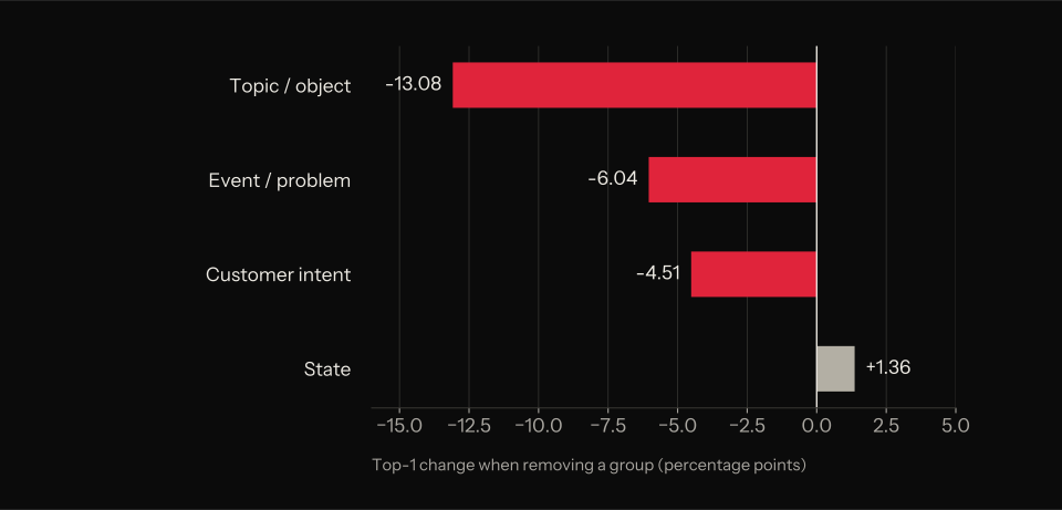
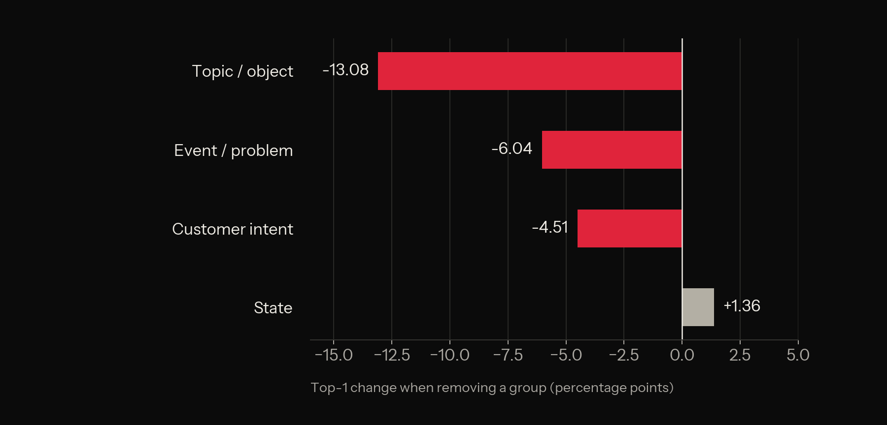
I removed one feature at a time and one entire group at a time. This is called an ablation: examining what happens when part of the system is removed. The analysis used weighted relevance, with the same model assessments and unchanged weights for the remaining features.
| Removed group | Top-1 | Change from the full weighted method |
|---|---|---|
| None | 28.02% | — |
| What the message concerns | 14.94% | −13.08 percentage points |
| Event or problem | 21.98% | −6.04 percentage points |
| What the customer wants | 23.51% | −4.51 percentage points |
| State | 29.38% | +1.36 percentage points |
The features describing what the message concerns had the largest combined effect. Removing the state group, however, produced a small Top-1 improvement. More features were therefore not automatically better with this ranking method.
This does not tell us which groups matter most for cosine. Nor does it mean that a feature with a small ablation effect is useless; another feature may carry much of the same information. All 38 ablations are documented, but they were not used to select a new schema and present the same test set as a fresh, untouched evaluation.
Cost and reproducibility
The study comprised 13,183 completed logical model calls: one for each of the 13,083 messages and 100 to interpret supplemental queries. One call required an additional attempt. The vectors were reused across the ranking methods, control tests, and ablations.
The JEV dashboard showed a total cost of USD 2.0765, or approximately 2.08 dollars, for the Jevbeddings project. The cost evidence and documentation are included with the research material.
All text fingerprints and saved feature values for the 13,083 messages were checked. A separate full sort for 31 fixed test queries produced the same top ten and first-relevant-result rank in all 124 method checks. The 25 automated program tests also passed.
The data source is pinned to commit 57ec275d8078af65b7731c2a98be812d844a6d6b. Code, protocol, questions, weights, per-query results, and saved model assessments are included in the reproduction package. This makes it possible to recalculate the rankings without new model calls. A fresh API extraction is a separate experiment; I do not guarantee identical answers from an external service over time.
What the study supports
In this experiment, 34 named features worked fairly well on BANKING77 when I used cosine similarity. The first result was correct more often than with BM25. With dot product, the same values performed substantially worse. This was one of the clearest findings: the ranking method mattered a great deal, even though the features were identical.
The supplemental queries also show that explicit feature requirements can be useful in this setup. At the same time, results weaken when natural language must first be translated into requirements, and the negative controls show that a numerically correct rule can still produce incorrect results.
Several questions remain unanswered. I tested one English-language banking dataset. I do not know whether JEV has previously seen BANKING77. The features are not calibrated against human judgments, and the retrieval tasks outside the main test are constructed from the categories. I also did not run a conventional embedding model as a comparator.
A follow-up study should therefore test the same idea on new messages, with independent judgments of both features and relevance, and with an embedding model as a baseline. Any changes made after this study must be evaluated on new test data.
For me, the experiment produced a concrete result to build on. I could trace a retrieved result down to each feature's contribution, and one ranking method worked well on this dataset. I could also see where the setup failed. Whether it works equally well on other types of text remains to be tested.
Sources and material
The data and results are included in the package. The evidence overview explains how to reproduce the calculations without new API calls and the limitations of local call logs and timestamps as evidence of the run itself.
- Casanueva, I., Temčinas, T., Gerz, D., Henderson, M., and Vulić, I. (2020). Efficient Intent Detection with Dual Sentence Encoders. BANKING77 dataset and license. The dataset is used under CC-BY-4.0; original labels are preserved.
- TypeSafe. JEV API and model reference. Model used in the experiment:
jev-1.13.0. - jevbeddings. Frozen protocol, implementation clarifications, run instructions, and feature schema.
- jevbeddings. Technical results report, machine-readable results, contributions to individual results, post-hoc analysis of winning documents, and verification calculations.
- Complete original reproduction archive. This historical snapshot retains the Norwegian documentation; the repository contains the English edition.
Run the numbers yourself.
The research archive contains code, datasets, saved model assessments and per-query results. Recalculate the results without an API key. The original archive retains its Norwegian documentation.
Download the complete experiment · 5.8 MB ↓Code, data and reproduction on GitHub ↗
What the evidence does and does not prove
All results (JSON) · Main results (CSV) · Study (English Markdown)